ndtv_workshop.Rmd

---
title: "Temporal network tools in statnet: networkDynamic, ndtv and tsna"
author: "Skye Bender-deMoll"
date: "04/05/2016"
output:
  html_document:
    fig_width: 8
    highlight: kate
    theme: cosmo
    toc: yes
    css: custom.css
  pdf_document:
    toc: yes
---
```{r setup, include=FALSE,cache=FALSE}
library(knitr)
knitr::opts_chunk$set(comment='') #,cache=TRUE)
library(animation)
#library(printr)
```

![](http://skyeome.net/wordpress/wp-content/uploads/2015/05/proxTimeineWithInf.png)

# Introduction to this workshop

This workshop will explore the key features of the open-source R packages that `statnet` suite provides for working with dynamic (longitudinal) network data:

 * `networkDynamic`  (Butts, et al) extends the `network` package to provide data structures for edge, vertex, and attribute dynamics
 * `ndtv` (Network Dynamic Temporal Visualization) provides tools for visualizing and animating changing network structure
 * `tsna` provides basic temporal social network analysis statistics, in part by leveraging algorithms provided by the `ergm`, `relevent` and `sna` packages.
 * `networkDynamicData` includes several dynamic network data sets shared by multiple authors. 
 
 There is much more material in the workshop than we will be able to cover in three hours, so this document is also intended to serve as a reference as well. 
 
 This work was supported by grant R01HD68395 from the National Institute of Health.


## Workshop prerequisites

  * Familiarity with the R statistical software.  This tutorial does not cover basics of how to use and install R.
  * Functioning R installation and basic statnet packages already installed. (Instructions on installing R and statnet are located here https://statnet.org/trac/wiki/Installation.)  RStudio recommended. 
  * Familiarity with general network and SNA concepts
  * Experience with statnet packages and `network` data structures preferred but not necessary. (A tutorial providing "An Introduction to Network Analysis with R and statnet"" is located here: https://statnet.org/trac/wiki/Resources)
  * A working internet connection (we will install some libraries and download data sets)

# A Quick Demo

Lets get started with a realistic example. We can render a simple network animation in the R plot window (no need to follow along in this part) 

First we load the package and its dependencies.
```{r,message=FALSE,cache=FALSE}
library(ndtv)
```
Now we need some dynamic network data to explore. The package includes an example network data set named `short.stergm.sim` which is the output of a toy STERGM model based on Padgett's Florentine Family Business Ties dataset simulated using the `tergm` package. (Using the tergm package to simulate the model is illustrated in a later example.)  

```{r}
data(short.stergm.sim)
```

## Render a network animation in a plot window
If we want to get a quick visual summary of how the structure changes over time, we could render the network as an animation.

```{r,fig.keep='none',message=FALSE,results='hide',cache=TRUE}
render.animation(short.stergm.sim)
```

And then play it back in the R plot window as many times as we want
```{r,fig.show='hide',cache=TRUE}
ani.replay()
```


## Render a network animation as an interactive web page
We can also present a similar animation as an interactive HTML5 animation in a web browser. 
```{r,message=FALSE,results='hide',cache=FALSE}
render.d3movie(short.stergm.sim)
```

This should bring up a browser window displaying the animation.  In addition to playing and pausing the movie, it is possible to click on vertices and edges to show their ids, double-click to highlight neighbors, and zoom into the network at any point in time. 

## Render a network in markdown document or RStudio
By changing the output slightly, we can embed directly in an Rmarkdown document or RStudio plot window
```{r,message=FALSE,cache=FALSE}
render.d3movie(short.stergm.sim,output.mode = 'htmlWidget')
```


## Plot a static "filmstrip" sequence

An animation is not the only way to display a sequence of views of the network.  We could also use the `filmstrip()` function that will create a "small multiple" plot using frames of the animation to construct a static visual summary of the network changes.

```{r,cache=TRUE}
filmstrip(short.stergm.sim,displaylabels=FALSE)
```

## Plot a "timePrism" projection
If were to select some of the 'small multiple' frames from the movie and stack them up in layers of time, we will have an illustrative 'timePrism' projection of the network. This view introduces some clutter and distortion, but includes both some time and some relational information
```{r,message=FALSE}
compute.animation(short.stergm.sim)
timePrism(short.stergm.sim,at=c(1,10,20),
          displaylabels=TRUE,planes = TRUE,
          label.cex=0.5)
```


## Plot a timeline
If we want to focus solely on the relative durations of events, we can view the dynamics as a `timeline` by plotting the active spells of edges and vertices.
```{r}
timeline(short.stergm.sim)
```

In this view, only the activity state of the network elements are shown--the structure and network connectivity is not visible. The vertices in this network are always active so they trace out unbroken horizontal lines in the upper portion of the plot, while the edge toggles are drawn in the lower portion.  

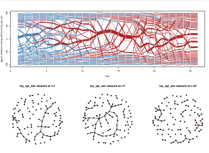
## Plot a proximity timeline
We are experimenting with a form of timeline or "phase plot". In this view vertices are positioned vertically by their geodesic distance proximity.  This means that changes in network structure deflect the vertices' lines into new positions, attempting to keep closely-tied vertices as neighbors. The edges are not shown at all in this view. 

```{r,message=FALSE,cache=TRUE}
proximity.timeline(short.stergm.sim,default.dist=6,
          mode='sammon',labels.at=17,vertex.cex=4)
```

Notice how the bundles of vertex lines diverge after time 20, reflecting the split of the large component into two smaller components. 

## Print tabular data

Of course we can always display the edge (or vertex) spells directly in a tabular form using the various utilities in the `networkDynamic` package. 

```{r}
head( as.data.frame(short.stergm.sim) )
```

*****
**Question:** What are some strengths and weakness of the various views?

*****

*****
**Exercise:** Load the saved version of `short.stergm.sim`. Are there any edges that are present for the entire time period from 0 until 25?


```{r}
data(short.stergm.sim)
spls<-as.data.frame(short.stergm.sim)
spls[spls$duration==25,]
```

*****

## Compute some basic temporal stats

Load up the `tsna` (Temporal Social Network Analysis) library
```{r,message=FALSE}
library(tsna)
```

How many edges form at each time step for the `short.stergm.sim`?  Conveniently, the values are returned as a time series, `plot` already knows how to handle them.
```{r}
tEdgeFormation(short.stergm.sim)

plot( tEdgeFormation(short.stergm.sim) )
```


## Compute static graph-level sna measure as a time series

The `tsna` package provides wrapper functions that make it easy to compute a time series using statistics from the `sna` package or `ergm` terms.  For example, we can use the `gtrans` function to compute transitivity in the network. 

```{r}
plot( tSnaStats(short.stergm.sim,'gtrans') )
```


## Find temporally reachable paths

We can quickly compute the earliest times a journey from vertex 13 can reach the rest of the network traveling forward along time-respecting paths in the network.  And then plot this path as an overlay on the aggregate network.

```{r}
path<-tPath(short.stergm.sim,v = 13,
            graph.step.time=1)

plotPaths(short.stergm.sim,
          path,
          label.cex=0.5)
```


# The Basics

Now that we've had a quick tour of some of what we will cover in the tutorial, lets get things set up and explain what is going on. 

## Installing the packages 

The `ndtv` (Bender-deMoll 2013) package relies on many other packages to do much of the heavy lifting, especially `animation` (Xie Y 2012) and `networkDynamic` (Butts et. al. 2012) which provides its input objects. Web animations can be created and viewed on computers with modern web browsers without additional components using the built-in `ndtv-d3` l.  However, `ndtv` does require some non-R external dependencies (`FFmpeg` or `avconv`) to save movies as video files, and Java to be able to use some of the better quality layout algorithms. These are discussed in a later section.

The core use-case for development is examining the output of statistical network models (such as those produced by the tergm (Krivitsky and Handcock 2015) package in statnet (Handcock et. al. 2003b) and simulations of disease spread across networks. The design philosophy is that it should be easy to do basic things, but lots of ability to customize.

R can automatically install the packages `ndtv` depends on when `ndtv` is installed. So open up your R console, and run the following command:
```{r,message=FALSE,results='hide'}
install.packages('ndtv',repos='http://cran.us.r-project.org', 
                 dependencies=TRUE)
library(ndtv) # also loads animation and networkDynamic
```

We will also use the `tsna` package for temporal SNA, so let's install and load that now as well.  It will bring along the `sna` and `ergm` packages

```{r,message=FALSE,results='hide'}
install.packages('tsna',repos='http://cran.us.r-project.org', 
                 dependencies=TRUE)
library(tsna)
```


## Understanding how networkDynamic works

Lets take quick tour of a `networkDynamic` object and work through some example in more detail to explain what is going on. Please follow along by running these commands in your R terminal. 


We are going to build a simple `networkDynamic` object "by hand" and then peek at its internal structure and visualize its dynamics. Note that the `networkDynamic()` command provides utilities for constructing dynamic networks from real data in various data formats, see some the later examples. 

### Activating a static network

First, we will create a static network with 10 vertices
```{r}
wheel <- network.initialize(10)
class(wheel)
```

Next we add some edges with activity spells.  The edges' connections are determined by the vector of `tail` and `head` vertex ids, and the start and ending time for each edge is specified by the `onset` and `terminus` vectors.
```{r}
add.edges.active(wheel,tail=1:9,head=c(2:9,1),onset=1:9, terminus=11)
add.edges.active(wheel,tail=10,head=c(1:9),onset=10, terminus=12)
```

Adding active edges to a network has the side effect of converting it to a `networkDynamic`. Lets verify it.

```{r}
class(wheel)
print(wheel)
```

Notice that the object now has a class of both `networkDynamic` and `network`.  All `networkDynamic` objects are still `network` objects, they just include additional special attributes to store time information.  The print command for `networkDynamic` objects includes some additional info about the time range of the network and then the normal output from `print.network`.


Once again, we can peek at the edge dynamics by transforming a view of the network into a `data.frame`.
```{r}
as.data.frame(wheel)
```

When we look at the output `data.frame`, we can see that it did what we asked. For example, edge id 1 connects the "tail" vertex id 1 to "head" vertex id 2  and has a duration of 10, extending from the "onset" of time 1 until the "terminus" of time 11. 

It is important to remember that `dynamicNetwork` objects are also static `network` objects.  So all of the `network` functions will still work, they will just ignore the time dimension attached to edges and vertices. For example, if we just `plot` the network, we see all the edges that ever exist (and realize why the network is named "wheel"). 
```{r}
plot(wheel)
```

### Extracting from a dynamic network

If we want to just see the edges active at a specific time point, we could first extract a snapshot view of the network at a single point in time and then plot it. 
```{r}
plot(network.extract(wheel,at=1))
```

But we can also extract a view of the network covering an interval of time.
```{r}
plot(network.extract(wheel,onset=1,terminus=5))
```


The `network.extract` function is one of the many tools provided by the `networkDynamic` package for storing and manipulating the time information attached to networks without having to work directly with the low-level data structures. The command `help(package='networkDynamic')` will give a listing of the help pages for all of the functions.   

*****
**Exercise:** Use the help function to determine the difference between the `network.extract()` and `network.collapse()` functions

*****

### Under the hood: spells and the 'activity' attribute

A potentially confusing point about the language we use when expanding from the static `network` object to a dynamic `networkDynamic` context is that "edge" now means something like "a container for all of the realizations of a tie between (usually a pair of) vertices". An "edge-spell" refers to a specific period of time over which the edge is known to be active. 

The edge-spells for each edge are stored in an attribute named `activity` as a two-column matrix of starting and ending times (which we refer to as "onset" and "terminus").  For many tasks, we would use higher-level methods like `get.edgeIDs.active()` but, we can access timing information directly using `get.edge.activity`.

Print the edge activity of edge ids 1 and 2
```{r}
get.edge.activity(wheel)[1:2]
```

So the `networkDynamic` object is not a big list of matrices for each discrete time point, and it is not even a list of networks. It can comfortably capture networks as multiple waves, but it can also store continuous time networks where each tie has its own timestamp.  The help page `?activity.attribute` is a good place to learn more detail about how the `networkDynamic` package represents dynamics.


Since the static plot, doesn't show us which edges are active when, lets annotate it by labeling edges with their onset and termination times so we can check that it constructed the network we told it to.

Make a list of labels for each edge, pasting the onset and terminus time together.
```{r}
elabels<-lapply(get.edge.activity(wheel),
                function(spl){
                  paste("(",spl[,1],"-",spl[,2],")",sep='')
                })
```

Plot the network, labeling each edge using the list of times.
```{r}
plot(wheel,displaylabels=TRUE,edge.label=elabels,
     edge.label.col='blue') 
```

*****
**Question:** Why is this edge labeling function not general enough for some networks? (Hint: do edges always have a single onset and terminus time?)

*****


Now lets render the network dynamics as a movie and play it back so that we can visually understand the sequence of edge changes. 
```{r,message=FALSE,fig.keep='none'}
render.animation(wheel) # compute and render
ani.replay()
```

Hopefully, when you play the movie you see a bunch of labeled nodes moving smoothly around in the R plot window, with edges slowly appearing to link them into a circle. Then a set of "spoke" edges appear to draw a vertex into the center, and finally the rest of the wheel disappears. An example of the animation rendered as a movie is located at http://statnet.org/movies/ndtv_vignette/wheel.mp4.

### Transforming between representations

Later sections of this tutorial give more complete examples of importing real network data from various formats.  For the moment, we can quickly through translating from one type of representation to another. 

******
**Excercise:**  If the three adjacency matrices below represent three time points of a network, what would the corresponding timed-edgelist representation be?
```
t0:       t1:       t2:
0 1 0     0 1 0     0 0 0
0 0 0     0 1 0     0 1 0
1 0 0     0 0 0     0 1 0
````

```{r}
# create a network object from each matrix
t0<-as.network(matrix(c(0,1,0,
                        0,0,0,
                        1,0,0),ncol=3,byrow=TRUE))

t1<-as.network(matrix(c(0,1,0,
                        0,1,0,
                        0,0,0),ncol=3,byrow=TRUE))

t2<-as.network(matrix(c(0,0,0,
                        0,1,0,
                        0,1,0),ncol=3,byrow=TRUE))
# convert a list of networks into networkDynamic object
tnet<-networkDynamic(network.list=list(t0,t1,t2))
# print the networkDynamic object as a timed edgelist
as.data.frame(tnet)[,1:4]

```

******

******
**Excercise:**  Create a `networkDynamic` object from the timed edgelist below. Assume columns are onset, terminus, tail, head.

```
0	1	3	1
0	2	1	2
2	3	3	2
```
```{r}
tel<-matrix(c(0,1,3,1,
              0,2,1,2,
              2,3,3,2),ncol=4,byrow=TRUE)
tnet<-networkDynamic(edge.spells=tel)
```

******

### Data utilities 

The `networkDynamic` package provides many utilities for querying, constructing, and manipulating dynamic network data. Since we won't have time to delve into them all here, I'll just point out some of the help topics for features that may be easy to overlook, and suggest referring to the help index and `browseVignette(package='networkDynamic')`.

* `?networkDynamic` Convert various forms of network timing information (including toggles and matrices) into networkDynamic objects
* `?adjust.activity` Adjust and transform the activity ranges in all of the spells of a networkDynamic object.
* `?persistent.ids` Create and query 'persistent ids' of networks that will remain constant as network size changes due to extraction.
* `?reconcile.activity`  Clean up messy input data by modifying the activity spells of vertices to match incident edges or the other way around.
* `?timeProjectedNetwork`  Construct a time-projected ("multi-slice") network representation by binning a longitudinal network and linking time points with "identity arcs".
  
## Understanding how ndtv works

As we saw in the wheel example, creating the animations is simple right? Hopefully most of the complexity was hidden under the hood, but it is still useful to understand what is going on. At its most basic, rendering a movie consists of four key steps:

1. Determining appropriate parameters (time range, aggregation rule, etc)
2. Computing layout coordinates for each time slice
3. Rendering a series of plots for each time slice
4. Replaying the cached sequence of plots (or writing to a file on disk)

When we called `render.animation()` we asked the package to create an animation for `wheel` but we didn't include any arguments indicating what should be rendered or how, so it had to make some educated guesses or use default values. For example, it assumed that the entire time range of the network should be rendered and that we should use the Kamada-Kawai layout to position the vertices.
    
The process of positioning the vertices was managed by the `compute.animation()` function which stepped through the `wheel` network and called a layout function to compute vertex coordinates for each time step. 

Next, `render.animation()` looped through the network and used `plot.network()` to render appropriate slice network for each time step.  It calls the `animation` package function `ani.record()` to cache the frames of the animation. Finally, `ani.replay()` quickly redrew the sequence of cached images in the plot window as an animation.

The `render.d3movie()` works along the same lines, but in step three the 'render' it stores at each step is a description of the time slice in a web data language (JSON), and in step four it feeds the data into an web app (the ndtv-d3 player) which it then displays. 

### Controlling the animation processing steps

For more precise control of the processes, we can call each of the steps in sequence and explicitly set the parameters we want for the rendering and layout algorithms. First we will define a `slice.par`, which is a list of named parameters to specify the time range that we want to compute and render.

```{r}
slice.par=list(start=1, end=12, interval=1, aggregate.dur=1,
              rule='latest')
```

Then we ask it to compute the coordinates for the animation, passing in the `slice.par` list. The `animation.mode` argument specifies which algorithm to use.
```{r}
compute.animation(wheel,animation.mode='kamadakawai',slice.par=slice.par)
```

The x and y coordinates for plotting each time point are now stored in the network. 
```{r}
list.vertex.attributes(wheel)
# peek at x coords at time 4
get.vertex.attribute.active(wheel,'animation.x',at=4)
```

We can see that in addition to the standard vertex attributes of `na` and `vertex.names`, the network now has two dynamic "TEA" attributes for each vertex to describe its position over time. The `slice.par` argument is also cached as a network attribute so that later on `render.animation()` will know what range to render.

Since the coordinates are stored in the network, we can collapse the dynamics at any time point, extract the coordinates, and plot it:
```{r}
wheelAt8<-network.collapse(wheel,at=8)
coordsAt8<-cbind(wheelAt8%v%'animation.x',wheelAt8%v%'animation.y')
plot(wheelAt8,coord=coordsAt8)
```

This is essentially what `render.animation()` does internally.  The standard network plotting arguments are accepted by `render.animation` (via `...`) and will be passed to `plot.network()`:

```{r,fig.keep='none',message=FALSE}
render.animation(wheel,vertex.col='blue',edge.col='gray',
                 main='A network animation')
```

`render.animation()` also plots a number of in-between frames for each slice to smoothly transition the vertex positions between successive  points. We can adjust how many "tweening" interpolation frames will be rendered which indirectly impacts the perceived speed of the movie (more tweening means a slower and smoother movie). For no animation smoothing at all, set `tween.frames=1`.

```{r,fig.keep='none',message=FALSE}
render.animation(wheel,render.par=list(tween.frames=1),
                 vertex.col='blue',edge.col='gray')
ani.replay()
```

Or bump it up to 30 for a slow-motion replay:

```{r,fig.keep='none',message=FALSE}
render.animation(wheel,render.par=list(tween.frames=30),
                 vertex.col='blue',edge.col='gray')
ani.replay()
```

Note that the `render.d3movie` command doesn't have a `tween.frames` argument, because it interpolates the positions in the app. It has an `animationDuration` parameter that can be passed provided and an 'animation speed' control in the app which the use can adjust using the menu on the upper left. 

If you are like me, you probably forget what the various parameters are and what they do.  You can use `?compute.animation` or `?render.animation` to display the appropriate help files. and `?plot.network` to show the list of plotting control arguments.

*****
**Question:** Why is all this necessary? Why not just call plot.network over and over at each time point?

*****


### Animated Layout Algorithms
First some background about graph layouts.  Producing layouts of dynamic networks is generally a computationally difficult problem. And the definition of what makes a layout "good" is often ambiguous or very specific to the domain of the data being visualized. The ndtv package aims for the following sometimes conflicting animation goals:

* Similar layout goals as static layouts (minimize edge crossing, vertex overlap, etc)
* Changes in network structure should be reflected in changes in the vertex positions in the layout.
* Layouts should remain as visually stable as possible over time.
* Small changes in the network structure should lead to small changes in the layouts. 

Many otherwise excellent static layout algorithms often don't meet the last two goals well, or they may require very specific parameter settings to improve the stability of their results for animation applications. 

So far, in ndtv we are using variations of Multidimensional Scaling (MDS) layouts.  MDS algorithms use various numerical optimization techniques to find a configuration of points (the vertices) in a low dimensional space (the screen) where the distances between the points are as close as possible to the desired distances (the edges). This is somewhat analogous to the process of squashing a 3D world globe onto a 2D map: there are many useful ways of doing the projection, but each introduces some type of distortion. For networks, we are attempting to define a high-dimensional "social space" to project down to 2D.

The `network.layout.animate.*` layouts included in `ndtv` are adaptations or wrappers for existing static layout algorithms with some appropriate parameter presets. They all accept the coordinates of the previous layout as an argument so that they can try to construct a suitably smooth sequence of node positions. Using the previous coordinates allows us to "chain" the layouts together. This means that each visualization step can often avoid some computational work by using a previous solution as its starting point, and it is likely to find a solution that is spatially similar to the previous step. 


#### Why we avoid Fruchterman-Reingold
The Fruchterman-Reingold algorithm has been one of the most popular layout algorithms for graph layouts (it is the default for `plot.network`).  For larger networks it can be tuned to run much more quickly than most MDS algorithms.  Unfortunately, its default optimization technique introduces a lot of randomness, so the "memory" of previous positions is usually erased each time the layout is run, producing very unstable layouts when used for animations. Various authors have had useful animation results by modifying FR to explicitly include references to vertices' positions in previous time points. Hopefully we will be able to include such algorithms in future releases of ndtv.

#### Kamada-Kawai adaptation
The Kamada-Kawai network layout algorithm is often described as a "force-directed" or "spring embedded" simulation, but it is mathematically equivalent to some forms of MDS (Kamada-Kawai uses Newton-Raphson optimization instead of SMACOF stress-majorization). The function `network.layout.animate.kamadakawai` is essentially a wrapper for `network.layout.kamadakawai`. It computes a symmetric geodesic distance matrix from the input network using `layout.distance` (replacing infinite values with `default.dist`), and seeds the initial coordinates for each slice with the results of the previous slice in an attempt to find solutions that are as close as possible to the previous positions. It is not as fast as MDSJ, and the layouts it produces are not as smooth. Isolates often move around for no clear reason. But it has the advantage of being written entirely in R, so it doesn't have the pesky external dependencies of MDSJ. For this reason it is the default layout algorithm. 

```{r,message=FALSE,results='hide'}
compute.animation(short.stergm.sim,animation.mode='kamadakawai')
saveVideo(render.animation(short.stergm.sim,render.cache='none',
                           main='Kamada-Kawai layout'),
          video.name='kamadakawai_layout.mp4')
```

#### MDSJ (Multidimensional Scaling for Java)

MDSJ is a very efficient implementation of "SMACOF" stress-majorization Multidimensional Scaling. The `network.layout.animate.MDSJ` layout gives the best performance of any of the algorithms tested so far -- despite the overhead of writing matrices out to a Java program and reading coordinates back in.  It also produces very smooth layouts with less of the wobbling and flipping which can sometimes occur with Kamada-Kawai. Like Kamada-Kawai, it computes a symmetric geodesic distance matrix from the input network using `layout.distance` (replacing infinite values with `default.dist`), and seeds the initial coordinates for each slice with the results of the previous slice.

As noted earlier, the MDSJ library is released under Creative Commons License "by-nc-sa" 3.0.  This means using the algorithm for commercial purposes would be a violation of the license. More information about the MDSJ library and its licensing can be found at http://www.inf.uni-konstanz.de/algo/software/mdsj/.

```{r,echo=FALSE,message=FALSE}
# the command below will default to not installing MDSJ in a non-interactive session
# so to make sure it is installed for this sweave build, call it internally
mdsj.dir <- file.path(path.package("ndtv"), "java/")
ndtv:::install.mdsj(mdsj.dir)
```

```{r,message=FALSE,results='hide'}
compute.animation(short.stergm.sim,animation.mode='MDSJ')
saveVideo(render.animation(short.stergm.sim,render.cache='none',
                           main='MDSJ layout'),
          video.name='MDSJ_layout.mp4')
```

#### Graphviz layouts

The Graphviz (Gansner and North 2000)  external layout library includes a number of excellent algorithms for graph layout, including `neato`, an stress-optimization variant, and `dot` a hierarchical layout (for trees and Directed Acyclic Graph (DAG) networks). As Graphviz is not an R package, you must first install the the software on your computer following the instructions at `?install.graphviz` before you can use the layouts. The layout uses the `export.dot` function to write out a temporary file which it then passes to Graphviz.

```{r,message=FALSE}
compute.animation(short.stergm.sim,animation.mode='Graphviz')
saveVideo(render.animation(short.stergm.sim,render.cache='none',
                           main='Graphviz-neato layout'),
          video.name='gv_neato_layout.mp4')
compute.animation(short.stergm.sim,animation.mode='Graphviz',
                  layout.par=list(gv.engine='dot'))

```

#### Existing coordinates or customized layouts
The `network.layout.animate.useAttribute` layout is useful if you already know exactly where each vertex should be drawn at each time step (based on external data such as latitude and longitude), and you just want `ndtv` to render out the network. It just needs to know the names of the dynamic TEA attribute holding the `x` coordinate and the `y` coordinate for each time step. 

The `useAttribute` layout also provides an easy way to pass in static coordinates in order to create an animation to show edge changes with static vertex positions.  This can be handy for 'flipbook'-style animations and geographic map overlays.  

```{r,eval=FALSE}
staticCoords<-network.layout.kamadakawai(short.stergm.sim,layout.par = list())
activate.vertex.attribute(short.stergm.sim,'x',staticCoords[,1],onset=-Inf,terminus=Inf)
activate.vertex.attribute(short.stergm.sim,'y',staticCoords[,2],onset=-Inf,terminus=Inf)
compute.animation(short.stergm.sim,animation.mode='useAttribute')
```



It is also possible to write your own layout function and easily plug it in by defining a function with a name like `network.layout.animate.MyLayout`.  See the `ndtv` package vignette for a circular layout example `browseVignette(package='ndtv')`.

*****
**Excercise:** Compare the algorithms by watching the video outputs or watch this side-by-side composite version: http://statnet.org/movies/layout_compare.mp4. What differences are noticeable?

*****

```{r, cache=TRUE,echo=FALSE,results='hide'}
# use ffmpeg to composite the three videos into one
system(paste('ffmpeg -i ',ani.options("outdir"),'/MDSJ_layout.mp4', ' -i  ',ani.options("outdir"),'/kamadakawai_layout.mp4',' -i  ', ani.options("outdir"),'/gv_neato_layout.mp4', ' -filter_complex "[0:v:0]pad=iw*3:ih[bg]; [bg][1:v:0]overlay=w[both]; [both][2:v:0]overlay=w*2"  ',ani.options("outdir"),'/layout_compare.mp4',sep=''))
system(paste('xdg-open ',ani.options("outdir"),'/layout_compare.mp4',sep=''))
```

More detailed information about each of the layouts and their parameters can be found on the help pages, for example `?network.layout.animate.kamadakawai`.

## Understanding how tsna works

The `tsna` package currently provides four main classes of metrics

* Traditional SNA metrics evaluated repeatedly to return a time series
* Statistics describing properties of the network over its entire observation period
* Metrics based on measuring network distances using forward reachable paths
* Measures of event sequences

The first class of metrics requires some additional detail about how we think about dividing and aggregating time. 

### Slicing and aggregating time

Most traditional "static" network metrics don't really know what to do with dynamic networks.  They need to be fed a set of relationships describing a single point in time in the network's evolution which can then be used to compute graph metrics.   A common way to apply static metrics to characterize a time-varying object is to sample it at regular intervals, taking a sequence static observations at multiple time points and using these to describe the changes over time.  

In the case of networks, we often call this this sampling process "extracting" or "slicing" --cutting through the dynamics to obtain a static snapshot.  For the network layouts we want a sequence of these snapshots to be converted into series of coordinates in Euclidean space suitable for plotting. For graph- or vertex-level SNA indicators we want a time series of numeric values. The processes of determining a set of slicing parameters appropriate for the network phenomena and data-set of interest requires careful thought and experimentation.  As mentioned before, it is somewhat similar to the questions of selecting appropriate bin sizes for histograms.

#### Slicing panel data

In both the `wheel` and `short.stergm.sim` examples, we've been implicitly slicing up time in discrete way, extracting a static network at each unit time step.

We can plot the slice bins against the timeline of edges to visualize the "observations" of the network that the rendering process is using. When the horizontal line corresponding to an edge spell crosses the vertical gray bar corresponding to a bin, the edge would be included in that network. If this was a social network survey, each slice would correspond to one data collection panel of the network.  
```{r}
timeline(short.stergm.sim,slice.par=list(start=0,end=25,interval=1,
                      aggregate.dur=1,rule='latest'),
                      plot.vertex.spells=FALSE)
```

Looking at the first slice, which extends from time zero *until* (notice the right-open interval definition!) time 1, it appears that it should have 15 edges in it.  Let's check. We can either:

Extract the network as we have seen before and count edges...
```{r}
network.edgecount(network.extract(short.stergm.sim,onset=0,terminus=1))
```
... or just count the active edges directly with a command.
```{r}
network.edgecount.active(short.stergm.sim,onset=0,terminus=1)
```

If we want to do this for each slice, we can use the `edges` statistic from `ergm`

```{r}
tErgmStats(short.stergm.sim,'edges',start = 0,end=25,time.interval=1)
```


Following the convention `statnet` uses for representing ``discrete-time`` simulation dynamics, the edge spells always have integer lengths and extend the full duration of the slice, so it wouldn't actually matter if we used a shorter `aggregate.dur`. Each slice will still intersect with the same set of edges. 

```{r}
timeline(short.stergm.sim,slice.par=list(start=0,end=25,interval=1,
                      aggregate.dur=0,rule='latest'),
                      plot.vertex.spells=FALSE)
```


However, even for some data-sets that are collected as panels, the time units many not always be integers, or the slicing parameters might need to be adjusted to the natural time units.  For example, if we use `aggregate.dur` to specify longer duration bins, some of them will intersect with more edges


```{r,warning=FALSE}
tErgmStats(short.stergm.sim,'edges',start = 0,end=25,time.interval=2, aggregate.dur=2)
```

And, as we will see later in the windsurfers example, there are situations where using longer aggregation durations can be helpful even for panel data. 

#### Slicing streaming data

Slicing up a dynamic network created from discrete panels may appear to be fairly straightforward but it is much less clear how to do it when working with continuous time or "streaming" relations where event are recorded as a single time point. How often should we slice?  Should the slices measure the state of the network at a specific instant, or aggregate over a longer time period?  The answer probably depends on what the important features to visualize are in your data-set. One of the strengths of these packages is that they make it possible to experiment with various aggregation options. In many situations we have even found it useful to let slices mostly overlap -- increment each one by a small value to help show fluid changes on a moderate timescale instead of the rapid changes happening on a fine timescale (Bender-deMoll and McFarland 2006). 

As an example, lets look at the McFarland (2001) data of streaming classroom interactions and see what happens when we chop it up in various ways. 
```{r}
data(McFarland_cls33_10_16_96)
```

Plot the time-aggregated network
```{r}
plot(cls33_10_16_96)
```

First, we can animate at the fine time scale, viewing the first half-hour of class using instantaneous slices (`aggregate.dur=0`).
```{r,message=FALSE}
slice.par<-list(start=0,end=30,interval=2.5, 
                aggregate.dur=0,rule="latest")
compute.animation(cls33_10_16_96,
                slice.par=slice.par,animation.mode='MDSJ',verbose = FALSE)
render.d3movie(cls33_10_16_96,output.mode = 'htmlWidget')
```

Notice that although the time-aggregated plot shows a fully-connected structure, in the animation most of the vertices are isolates, occasionally linked into brief pairs or stars by speech acts. You can go to http://statnet.org/movies/ndtv_vignette/cls33_10_16_96v1.mp4 to see a version of the movie output. Once again we can get an idea of what is going on by slicing up the network by using the `timeline()` function to plot the `slice.par` parameters against the vertex and edge spells. Although the vertices have spells spanning the entire time period, in this data set the edges are recorded as instantaneous "events" with no durations.  

```{r}
timeline(cls33_10_16_96,slice.par=slice.par)
```

The very thin slices (gray vertical lines) (`aggregate.dur=0`) are not intersecting many edge events (purple numbers) at once so the momentary degrees are mostly low.  We can use the `ergm`'s `meandeg` term to compute the mean degree at each of the 50 time steps
```{r,warning=FALSE}
plot(tErgmStats(cls33_10_16_96,'meandeg'),
     main='Mean degree of cls33, 1 minute aggregation')
```


The first movie may give us a good picture of the sequence of conversational turn-taking, but it is hard to see larger structures. If we aggregate over a longer time period of 2.5 minutes we start to see the individual acts form into triads and groups. See http://statnet.org/movies/ndtv_vignette/cls33_10_16_96v2.mp4 for a version of the corresponding movie. 

```{r,message=FALSE}
slice.par<-list(start=0,end=30,interval=2.5, 
                aggregate.dur=2.5,rule="latest")
compute.animation(cls33_10_16_96,
                slice.par=slice.par,animation.mode='MDSJ',verbose=FALSE)
render.d3movie(cls33_10_16_96,
                 displaylabels=FALSE,output.mode='htmlWidget')
```

```{r}
timeline(cls33_10_16_96,slice.par=slice.par)
```

```{r,warning=FALSE}
plot(tErgmStats(cls33_10_16_96,'meandeg',
                time.interval = 2.5,aggregate.dur=2.5),
     main='Mean degree of cls33, 2.5 minute aggregation')
```

To reveal slower structural patterns we can make the aggregation period even longer, and let the slices overlap (by making `interval` less than `aggregate.dur`) so that the same edge may appear in sequential slices and the changes will be less dramatic between successive views. See http://statnet.org/movies/ndtv_vignette/cls33_10_16_96v3.mp4 for the corresponding movie.


```{r, message=FALSE}
slice.par<-list(start=0,end=30,interval=1, 
                aggregate.dur=5,rule="latest")
timeline(cls33_10_16_96,slice.par=slice.par)
compute.animation(cls33_10_16_96,
                slice.par=slice.par,animation.mode='MDSJ',verbose=FALSE)
render.d3movie(cls33_10_16_96,
                 displaylabels=FALSE,
               output.mode = 'htmlWidget')
```

```{r,warning=FALSE}
plot(tErgmStats(cls33_10_16_96,'meandeg',
                time.interval = 1,aggregate.dur=5,rule='latest'),
     main='Mean degree of cls33, overlapping 5 minute aggregation')
```

*****
**Question:** How would measurements of a network's structural properties (transitivity, betweenness, etc.) at each time point likely differ in each of the aggregation scenarios?

*****

*****
**Question:** When we use a long duration slice, for some networks it is quite likely that the edge between a pair of vertices has more than one active period. How should this condition be handled? If the edge has attributes, which ones should be shown? 

*****

Ideally we might want to aggregate the edges in some way, summing their activity durations or perhaps adding the weights together. Currently edge attributes are not aggregated and the `rule` element of the `slice.par` argument controls whether the `earliest` or `latest` attribute value should be returned for an edge when multiple elements are encountered.  

### The `ergm` and `sna` function wrappers

We've already seen several examples using the `tSnaStats` and `tErgmStats` functions.  These tools use the network statistics capabilities of the `sna` metrics and `ergm` terms  while handling the dirty work of chopping the `networkDynamic` object up into a series of appropriate `network`s (using `collapse.network`), interpreting some of the control parameters (directedness, etc), calculating the metric for each slice, and returning the results as time series (`ts`) object.  Be forewarned, this process is usually neither fast or memory efficient!  The binning of the networks is defined by the `time.interval` and `aggregate.dur` parameters, controlling the interval of time between the beginning of the bins and the duration of time that each bin aggregates. 

*****
**Exercise:** Define slicing parameters and compute a time series of graph `triad.census` values the first 20 minutes of classroom interactions using 5 minute non-overlapping slices 

```{r,warning=FALSE}
tSnaStats(cls33_10_16_96,'triad.census',
          start=0,
          end = 20,
          time.interval = 5, 
          aggregate.dur = 5)
```

*****

Notice that, unlike the previous temporal stats examples, the `triad.census` function returns multiple statistics -- the counts for each triad type -- and so `tSnaStats` returns a multivariate time series object in which each row is a time point and each column is one of the count statistics.

### Sequence measures

So far there is only one, `pShiftCount` which provides a wrapper for the implementation of Gibson's (2003) "participation shift" metric, provided by the `relevent` package (Butts, 2008). This measure considers the network to be an ordered sequence of events -- in which the exact timing is not important -- and tallies up instances of two-event exchanges into the thirteen categories Gibson used to classify conversational turn taking. 

For example, two edges in sequence, ‘i’ talks to ‘j’, and then ‘j’ responds to ‘i’, is counted as one type of event, where ‘i’ talks to ‘j’ and then ‘j’ talks to ‘k’ would be another type of event. The set of events Gibson was interested in is certainly not an exhaustive list of potential sequences, but may still be an interesting approach for characterizing dynamic networks.

If we apply the metric to the entire time period of the McFarland classroom speech acts

```{r}
pShiftCount(cls33_10_16_96)
```

We see lots of "turn-receiving" alternation (type AB-BA) and a fair amount of "turn-usurping" exchanges -- perhaps indicating time periods when multiple conversations are happening at the same time. 


Gibson's typology assumes that edges/ties directed "at the group" are distinguishable those directed to individuals, and has a strong assumption of sequential non-simultaneous events. Because the networkDynamic object does not explicitly code for 'group' utterances, simultaneous edges originating from a speaker (same onset, terminus, and tail vertex) are assumed to be directed at the group, even if not all group members are reached by the ties.

*****
**Question:** What are some key distinctions between the types of structures counted by `pShiftCount` when compared with a `triad.census`?

*****

### Durations and counts of ties

When we have access to longer duration longitudinal network data sets, it begins to be possible to examine networks in terms of temporal characterizations of edge activity without first chopping them up into bins.  For example, what are the average durations of edge activity?

The `edgeDuration` function provides a convenient way to access the information.

```{r}
edgeDuration(short.stergm.sim)
```
By default, it returns a vector of durations corresponding to each edge observed in the network. We can use standard R tools to look at these distributions. 

```{r}
summary( edgeDuration(short.stergm.sim) )
```

If we are working with event data such as the McFarland classrooms, this function at first appears less useful:

```{r}
edgeDuration(cls33_10_16_96)
```

Fortunately, there is an argument appropriate for working networks having zero-duration ties: instead of summing the duration of edges' activity spells, we tell it to just count the number of times they are active. 

```{r}
edgeDuration(cls33_10_16_96,mode='counts')
```

An important point of detail: when we compute statistics and the level of an 'edge', we are usually summing together all of the activity spells associated with that edge. Setting `subject = 'spells'` will return a duration for each edge activity spell, which is probably more consistent with what statistical models such as `tergm` consider the duration of an `edge`. For multiplex networks, setting `subject = 'dyads'` will aggregate across multiple edges linking a pair of vertices.  

```{r}
hist(edgeDuration(short.stergm.sim))  
hist(edgeDuration(short.stergm.sim,subject = 'spells')) 
```

****
**Question:** What happens to the measured durations as the observation window gets shorter? Why?

```{r}
summary(edgeDuration(short.stergm.sim))
summary(edgeDuration(short.stergm.sim,start=0,end=10))
```

****

Edge durations can tell us the relative rates at which individual relationships are active, but what if we want to know how active the vertices are across their relationships?  The `tiedDuration` function provides a vertex-level aggregation of the amount of time each vertex is "in a relationship".

```{r}
tiedDuration(short.stergm.sim)
```

****
**Question:** What might be an expected relationship between the `tiedDuration` and the `degree` of each vertex in a dynamic network?

****


### Forward path metrics
In static networks we frequently measure distances using the shortest path geodesic.  In dynamic networks that are models of possible transmission routes, we need to consider the sequence of edge timing when computing allowable 'journeys' through the network. The `tPath` function provides a way to calculate the set of temporally reachable vertices from a given source vertex starting at a specific time. 

```{r}
path<-tPath(short.stergm.sim,v = 13,
            graph.step.time=1)
path
```

By default, it does this by computing the `earliest forward reachable path`, so it also returns the earliest times each of the vertices becomes reachable in the `$tdist` component of the list, with `Inf` if it was unreachable.  The  `$previous` component gives, for each vertex, the id of the vertex it was reached by.  `$gsteps` gives the number of steps in the earliest forward path journey to reach each vertex. Note that this __is usually not the same thing as the length of the shortest time-respecting path!__ 

We showed previously that we plot the tPath overlayed on the aggregate network with `plotPaths`, but this is probably only useful when the aggregate network is not too dense. So another option is to just plot the tree of the reachable path as if it was a network. By default this will label the edges with the times that the path crossed them. 

```{r}
plot(path,edge.lwd = 2)
```

The `transmissionTimeline` is an alternate view which is often helpful for debugging and understanding tPaths. It plots the time at which each vertex was reached against the number of steps in the path with lines corresponding to the edges that the path crossed.

```{r}
transmissionTimeline(path,jitter=TRUE,
          main='Earliest forward path from vertex 13')
```

****
**Question:** Are reachable paths symmetric in an undirected network? If vertex `i` can reach `j`, can we assume that `j` can reach `i`?

****

Because reachable paths are not symmetric, the idea of "components" is much more complex in dynamic networks.  However, we can use the reachable paths to find the sizes of the 'forward reachable sets' from each vertex in the network with the `tReach` function.  This corresponds to the distribution of maximal possible epidemic sizes for a trivial SI infection model with a transmission probability of 1.0, so may give us a possible measure of how effective the network might be at transmitting. 

If we compute this for the `short.stergm.sim`, we will get back a vector where each element holds the reachable set size of the corresponding vertex -- starting from the beginning of the observation period.

```{r}
tReach(short.stergm.sim)
```

This tells us that the example network is fairly well temporally connected.  Most of the vertices can eventually reach at least 11 other vertices within the period of time we have "observed". For a network this small, we can efficiently compute all of the paths.  But for larger networks we might want to just get a sense of the distribution of forward set sizes using the `sample` argument to only compute paths from a subset of seed vertices. 


# Using the tools effectively
Some additional tips, tricks, and helpful information for temporal visualization.

## Animation output formats for ndtv
In this tutorial we have been only playing back animations in the R plot window. But what if you want to share your animations with collaborators or post them on the web? Assuming that the external dependencies are correctly installed, we can save out animations in multiple useful formats supported by the `ndtv` and the `animation` package:

* `render.d3movie()` plays an HTML5 vector graphics version of the animation in a browser window, Rmarkdown, or optionally saves it for later embedding.
* `ani.replay()` plays the animation back in the R plot window. (see `?ani.options` for more parameters)
* `saveVideo()` saves the animation as a video file on disk (if the FFmpeg library is installed).
* `saveGIF()` creates an animated GIF (if ImageMagick's  `convert` is installed)
* `saveLatex()` creates an animation embedded in a PDF document

See the help page for each function for detailed listing of parameters. We will quickly demonstrate some useful options below.

### HTML5 / SVG video files

As we saw earlier, `ndtv` includes the `render.d3movie` that, instead of using R's plotting functions and the animation library, embeds the animation information into a web page along with "ndtv-d3 player" as an interactive HTML5 SVG animation for display in a modern web browser.


```{r,message=FALSE}
render.d3movie(wheel,vertex.col='blue', edge.col='gray')
```

The `render.d3movie` supports most (but not all) of the same commonly used plot arguments as `render.animation`. For a list of exactly which arguments, see `?render.d3Movie`.  There are also some additional arguments that can be used to configure HTML styling and interaction properties such as tool-tips. 

We've provided a tutorial devoted just to the ndtv-d3 features available at http://statnet.org/workshops/SUNBELT/current/ndtv/ndtv-d3_vignette.html  It demonstrates great features such as embedding animations in Rmarkdown documents (Allaire, et. al. 2015) such as this tutorial, and some of the features that may be useful for building Shiny apps. 


### Video files
Since we just rendered the "wheel" example movie, it is already cached and we can capture the output of `ani.replay()` into a movie file. Try out the various output options below.

#### Saving video
Save out an animation, providing a non-default file name for the video file:

```{r,message=FALSE}
saveVideo(ani.replay(),video.name="wheel_movie.mp4")
```

You will probably see a lot output on the console from ffmpeg reporting its status, and then it should open the movie in an appropriate viewer on your machine.

#### Changing video size
Sometimes we may want to change the pixel dimensions of the movie output to make the plot (and the file size) much larger.
```{r,message=FALSE}
saveVideo(ani.replay(),video.name="wheel_movie.mp4",
          ani.width=800,ani.height=800)
```

#### Adjusting video quality
We can increase the video's image quality (and file size) by telling ffmpeg to use a higher bit-rate (less compression) for the video.

```{r,message=FALSE}
saveVideo(ani.replay(),video.name="wheel_movie.mp4",
          other.opts="-b:v 5000k")
```

#### Rendering video directly to disk
Because the `ani.record()` and `ani.replay()` functions cache each plot image in memory, they are not very speedy and the rendering process will tend to slow to a crawl down as memory fills up when rendering large networks or long movies.  We can avoid this by saving the output of `render.animation` directly to disk by wrapping it inside the `saveVideo()` call and setting `render.cache='none'`.
```{r,message=FALSE}
saveVideo(render.animation(wheel,vertex.col='blue',
          edge.col='gray',render.cache='none'),
          video.name="wheel_movie.mp4")
```

### Animated GIF files
We can also export an animation as an animated GIF image. GIF animations will be very large files, but are very portable for sharing on the web. To render a GIF file, you must have ImageMagick installed. See `?saveGIF` for more details. 

```{r,message=FALSE,results='none'}
saveGIF(render.animation(wheel,vertex.col='blue',
          edge.col='gray',render.cache='none'),
         movie.name="wheel_movie.gif")
```

### Animated PDF/Latex files
The `animation` package supports including animations inside PDF documents if you have the appropriate Latex utilities installed. However, the animations will only play inside Adobe Acrobat PDF viewers so it is probably less portable than using GIF or video renders.

```{r,message=FALSE}
saveLatex(render.animation(wheel,vertex.col='blue',
          edge.col='gray',render.cache='none'))
```



*****
**Exercise:** Using the list of options from the help page `?ani.options`, locate the option to control the time delay interval of the animation, and use it to render a video where each frame stays on screen for 2 seconds.

```{r,message=FALSE,results='hide'}
saveVideo(render.animation(wheel,vertex.col='blue',
          edge.col='gray',render.cache='none',
          render.par=list(tween.frames=1),
          ani.options=list(interval=2)),
         video.name="wheel_movie.mp4")
```

*****

*****
**Exercise:** Using the list of options from the help page `?render.d3movie`, locate the option to control the title and background color and load an animation in the web browser with the `d3.options` set so that it will play automatically, with a much faster duration than normal.

```{r,message=FALSE,results='hide'}
render.d3movie(wheel,vertex.col='blue',
          main="I'm a wheel!",
          bg='gray',
          d3.options=list(animationDuration=100,animateOnLoad=TRUE))
          
```

*****

*****
**Question:** What are some trade-offs between the HTML5 and video approaches to saving and sharing network animations?

****

## Vertex dynamics
In some dynamic network data the vertices may also enter or leave the network (become active or inactive, birth/death).  Lin Freeman's windsurfer social interaction data-set (Almquist and Butts 2011) is a good example of this. Vertices enter and exit frequently because different sets of people are present on the beach on successive days. For instance, look at vertex 74 in contrast to vertex 1 on the timeline plot.

```{r}
data(windsurfers)
timeline(windsurfers,plot.edge.spells=FALSE)
```


```{r,message=FALSE}

slice.par<-list(start=1,end=31,interval=1, 
                aggregate.dur=1,rule="earliest")
windsurfers<-compute.animation(windsurfers,slice.par=slice.par,
                               default.dist=3,
                               animation.mode='MDSJ',
                               verbose=FALSE)

render.d3movie(windsurfers,vertex.col="group1",
                 edge.col="darkgray",
                 displaylabels=TRUE,label.cex=.6,
                 label.col="blue", verbose=FALSE,
               main='Windsurfer interactions, 1-day aggregation',
               output.mode = 'htmlWidget')

```

These networks also have a lot of isolates, which tends to scrunch up the rest of the components in the network plot so they are hard to see.  Setting the lower `default.dist` above can help with this. In this example (see http://statnet.org/movies/ndtv_vignette/windsurfers_v1.mp4) the turnover of people on the beach is so rapid that structure appears to change chaotically, and it is quite hard to see what is going on. Notice the blank period at day 25 where the network data is missing.

We can still calculate some vertex-level metrics, such as the activity durations for each vertex. 

```{r}
hist( vertexDuration(windsurfers) )
```

Not surprisingly, most of the windsurfers spend less than 5 days a month on the beach. 

*****
**Question:**  What is the difference between calculating the vertex durations with `subject='vertices'` and `subject='spells'`? 

*****

What is happening to the density of the network as vertices enter and exit? Should we be thinking of the vertices as inactive, or unobserved?

```{r}